ISSN 1884-0760
GRACE TECHNICAL REPORTS
iGRT: A Generic Interface for GRoundTram
Yiqing ZHU Tao ZAN
Soichiro HIDAKA Zhenjiang HU
GRACE-TR 2012–06 June 2012
CENTER FOR GLOBAL RESEARCH IN
iGRT: A Generic Interface for GRoundTram
Yiqing ZHU1
Tao ZAN2
Soichiro HIDAKA3
Zhenjiang HU3
1
School of Software, Shanghai Jiao Tong University, China
The Graduate University for Advanced Studies, Japan
National Institute of Informatics, Japan
{hidaka, hu}@nii.ac.jp
June 5th, 2012
Abstract
Bidirectional transformation plays an important role in maintaining the consistency of two models, and it has many potential applications, such as model synchronization, software evolution, etc. Currently we have a powerful tool called GRoundTram, which is designed for compo-sitional development of well-behaved and efficient bidirectional graph transformations. However, as the graph representation in GRound-Tram is a directed edge-labelled graph, it is quite difficult to apply it to real-world graphs directly, as graphs have more sophisticated repre-sentations usually.
In this paper, we present iGRT, a generic interface for GRound-Tram. It serves as the connection between the graphs in real world and GRoundTram system. We have designed the representation for real world graphs, and provided traceable transformations between real-world graph representation and GRoundTram representation without losing any information. By using iGRT, we can easily shuttle between the different representations and maintain the synchronization as well. We have implemented iGRT and offered a friendly user interface based on the eclipse framework. Experiment result shows that iGRT en-hances GRoundTram’s application work to a large extent.
1
Introduction
From Wikipedia, “bidirectional transformations (bx) are programs whose code expresses a transformation both from input to output and back to the
corresponding input (possibly with modifications) in a single piece of code”.1
It aims at maintaining the consistency of two (or more) related sources of information, especially for software engineering domains [5].
It has been realized nowadays thatbx can provide solutions to a diverse
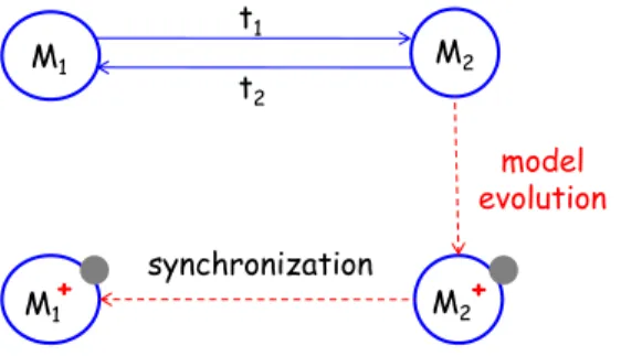
set of problems, such as model synchronization, software evolution, etc [12]. Figure 1 shows one example in model-driven software development.
Sup-pose M1 and M2 are two models, and there already exists one bx (t1 and
t2) between them. t1 is a transformation from M1 to M2, and t2 is the
corresponding backward transformation. From the picture we can see that
once M2 has evolved to M2+
with some modifications (signified as the grey
part in M2+), by using the transformation t2, we can easily get the relevant
evolved model M1+
, with the reflected modifications on M1 (signified as the
grey part in M1+
), thus keeping the synchronization of the two models.
M1 M2
M1+ M2+
model evolution t1
t2
synchronization
Figure 1: Model evolution by bidirectional transformation.
Currently, we have developed a powerful tool called GRoundTram [9] [11]. It is an integrated framework for developing well-behaved bidirectional
model transformations, and it also provides bx on graphs [7] [6] [10] [4].
Bidirectional graph transformation has long been regarded as an important but difficult problem, because a large part of the objects in real world can be modeled as graphs, while treating graphs is more difficult than treating trees, as it has a more complicated structure which contains cycles. By using GRoundTram, graphs can be processed so that operations such as queries and transformations can be done quite efficiently on graphs. Figure 2 is the overview of the GRoundTram system. It is composed of four main parts,
input, validation, bx and graphic user interface. The input to the system
is a source model together with its schema, a transformation described in
UnQL+
, and a target model schema. The validation part serves as a mecha-nism to detect errors during development as early as possible and help users
to develop correct models and transformations. Thebxpart makes
GRound-Tram unique as it provides well-behaved bidirectional transformation, and it also provides a user-friendly GUI to make itself easily used. Readers can refer to the user manual of GRoundTram [8] for more information.
!"#"$%&'"()*+, -$*)./($0*'"()
Source Model (DOT/UnCAL)
Source Schema (KM3)
Model Validation
Forward Transformation
Transformation (UnQL+)
Target Schema (KM3)
Model Transformation Validation
Verified Transformation
Target Model (DOT)
Graph Update
Updated Target Model (DOT) Backward
Transformation Updated Source Model
(DOT) Graph Update Source Model
(DOT)
Figure 2: Overview of GRoundTram.
the internal graph representation in GRoundTram is directed edge-labeled graph [3], and it is not a direct representation for most graphs in real world as they usually hold information on nodes. For example, the edge may be directed or undirected, and the node may also have labels.
Such shortage will lead to the fact that GRoundTram cannot be eas-ily applied to most common graphs, as the different representations of the graphs in two parts have placed a big obstacle between real world and
GRoundTram. Therefore, the ability of this powerful tool to process bx
on graphs has been decreased a lot.
In this paper, we present iGRT, a generic interface for GRoundTram.
It provides a way to make GRoundTram more applicable by giving transfor-mations between general graphs and internal graphs in GRoundTram. By taking advantage of iGRT, users can easily shuttle between the two kinds of graphs without losing any information, thus being able to use GRound-Tram to treat general graphs in real world directly. For example, giving two real-world graphs with general representation, we can first use iGRT to transform them into GRoundTram graphs, and then use GRoundTram to transform them with each other. When finishing processing these graphs, we can use iGRT to transform them back to general graphs with reflected modification or other impact on the original ones. In this way, a connection between these two real-world graphs has been created.
com-mon attributes and structures from them, therefore designed methodology for processing general graphs. Here we have selected three specific graphs:
usecasediagram,classdiagram andstatediagram. The former two are very
popular graphs from UML diagrams. They are quite necessary in software
development process. Andstatediagram is also very common for it models
the behaviour of a system, specifying the sequence of events that a system goes through during its lifetime in response to events. Due to the represen-tativeness of these three graphs, the common attributes and transformation methodology concluded from them can be well applied to most graphs in real world.
The rest of the paper is organized as follows: the next section presents the overview of iGRT. Section 3 illustrates how to represent general graphs in real world as well as in the GRoundTram system. The transformation algorithms between these two kinds of graphs are explained in Section 4. Meanwhile, the representations and algorithms for the three specific graphs will also be shown as concrete examples along with the description for general graphs in these two sections. Some useful operations based on iGRT such as graph modification propagating and graph query propagating which can be used to support solving the updating problem between real-world graphs and GRoundTram graphs will be described in Section 5. Section 6 gives the technical details of the implementation of iGRT, and Section 7 concludes the paper.
2
Overview
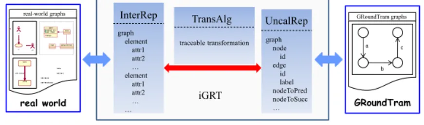
Figure 3 shows an overview of our approach. As can be seen from the picture, iGRT has three main parts: InterRep, TransAlg and UncalRep. The two outside mediums of iGRT are real-world graphs and GRoundTram graphs, and our work seems like a middleware connecting real world and the GroundTram system. Now let us have a first look at how iGRT behaves.
UncalRep iGRT InterRep TransAlg … ….. …… ……… real-world graphs u1 u2 uc open close safe closed GRoundTram GRoundTram graphs a b c graph element attr1 attr2 … element attr1 attr2 … …
traceable transformation graph node id edge id label nodeToPred nodeToSucc … real world
Figure 3: Overview of iGRT.
they are always saved in distinct formats, such as XML [2], dot, etc. In order to treat various graphs using the same methodology, we need to unify them into a solitary representation. The InterRep part is responsible for this unification work. Given a real-world graph as input, InterRep part will nor-malize it with the specified graph schema . We have defined several default schemas for some popular graphs, and the schemas can also be provided by the users. According to the schema, different graphs can be unified into the same intermediate representation (InterRep graph), thus being able to be treated in one way.
As pointed out before, the GRoundTram system has its internal graph representation which is directed graph with edge labeled. Serving as a con-nector connecting GRoundTram with real world, iGRT also has another part, UncalRep, targeting at representing the graphs in GRoundTram. The graph representation in UncalRep (UncalRep graph) is quite similar to graphs in GRoundTram, other than it may contain some additional at-tributes to make the transformation algorithms work more conveniently, such as “nodeToSucc” attribute, which signifies the succeeding nodes of each node.
So far iGRT already has two parts representing the graphs in real world and GRoundTram. What we need now is a way to shorten the distance be-tween them. This work is done by the TransAlg part. In this part, we have presented traceable transformation algorithms, on purpose of doing trans-formation between InterRep graphs and UncalRep graphs bidirectionally without losing any information. “traceable” here specifies that the algo-rithms will save the trace information when doing the transformation work [13]. Therefore, when one graph has been transformed to another graph by these algorithms, it can be traced back to the original one directly.
In addition, according to the saved trace information, when one graph is updated with some modifications, the modifications can be easily propagated to the other graph by some additional operations based on the trace, such as modification propagating and query propagating, so that the two graphs can be kept synchronized. Moreover, graph query can also be transferred from InterRep graph to UncalRep graph. When users want to do query on real-world graph, the query will be translated onto the corresponding graph in GRoundTram system, hence the query task can be fulfilled by GRoundTram.
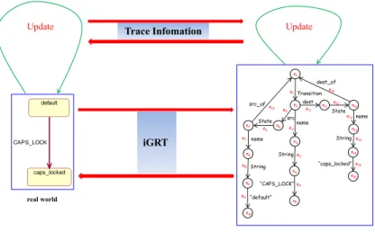
Figure 4 is a usage scenario of our work. From the picture we can see that iGRT stands between real world and the GroundTram system. If we want to
use GRoundTram to treat some real-world graph, say onestatediagram in
State State Transition String src dest name e1 n1 src_of “CAPS_LOCK”e4 String “default” dest_of name String “caps_locked” n2 name n3 n4 n5 n6 n7 n8 n9 n10 n11 n12 n13 n14 n15 e2 e3 e5 e6 e7 e8 e9 e10 e11 e12 e13 e14 e15 e16 default caps_locked CAPS_LOCK iGRT real world GRoundTram Update Trace Infomation Update
Figure 4: Usage scenario of iGRT.
part to the left part is quite similar. And due to the saved trace information, when there are some modifications on the InterRep graph, the modifications will be directly propagated to the UncalRep one. For example, after iGRT transforms the state diagram to the edge-labeled graph, if the edge labeled “CAPS LOCK” has been changed to edge labeled “CAPS UNLOCK” when GRoundTram does some operations on the graph, the iGRT will transfer the modification back to the original state diagram according to the trace information. As a result, the transition “CAPS LOCK” will be evolved to transition “CAPS UNLOCK”.
iGRT is developed based on the Eclipse platform, and all the graphs and algorithms are coded in Java. The detailed techniques about the imple-mentation will be discussed in Section 6. In the next section, we will first explain the working mechanism of the InterRep part and the UncalRep part in iGRT.
3
InterRep and UncalRep in iGRT
3.1 General InterRep and UncalRep Graph
Generally speaking, graphs are composed of nodes and edges, and they have their own properties with different types. Here we will first generalize graphs by regarding all their contents as elements and attributes. More specifically, all the nodes and edges in the graph are considered as “element”. And their properties are thought of as the “attribute” of the “element”. Moreover, if the type of the property is reference rather than primitive, the property itself also becomes an “element”, according to this mechanism, the type of the “attribute” will be primitive or “element”.
In this way, we can easily normalize the real-world graph in the following schema, and it is also the cornerstone of iGRT’s InterRep part. Here the language for specifying graph schemas is similar with KM3 [1], a neutral language to write metamodels and to define domain specific languages. From the schema we can see that the graph may contain several elements. Each
element may contain several attributesaiwhose type is another element. By
using “ Primitive” to specify some primitive element such as string. “number = ...” signifies the number of this attribute that the element can hold.
Schema S = {
Element PrimitiveE1;
Element PrimitiveE2;
...
ElementEi {
attributea1 : Ej[number];
attributea2 : Ek[number];
...
}
ElementEi+1 {
attributea1 : Ej[number];
attributea2 : Ek[number];
...
}
...
}
schemas embedded in iGRT. After the graph and its schema being offered, InterRep part will automatically give the corresponding schema instance,
i.e. the InterRep graph in the following style. Notice that ei are elements
of the relevant graph schema, and ai are their attributes.
Instance iof S = {
ei1 ={
a1 = ...;
a2 = ...;
...
}
ei2 ={
a1 = ...;
a2 = ...;
...
}
...
}
The attained InterRep graph will then be transformed to UncalRep graph by iGRT’s TransAlg part. In this section we will not explain how the algorithm works, instead, we will first show the relevant UncalRep graph.
As the graph schema has signified clearly all the properties of the cor-related graph, and iGRT should not lose any information while doing the transformation, the UncalRep graph can be just created according to each element and its attributes by extending them to one branch in the Uncal-Rep graph. In detail, for each element, we will use one edge labeled with its name to represent the element itself. For each of its attribute, if it is primitive type, we will use three edges labeled with its name, type and the attribute itself to represent the attribute, and if it is “element” type, we will use one edge to label its name and then connect it with the corresponding element. In this way, the labels of the edges in the UncalRep graph can capture all the properties of the InterRep graph. Because UncalRep graph is quite similar to the internal graph representation in GRoundTram, it can be directly transferred to the graph that can be input to the GRoundTram system.
3.2 Concrete Cases
A. Use Case Diagram
In the Unified Modeling Language, use case diagram overviews the usage requirements for a system. They are useful for presentations to management and/or project stakeholders as well as developers.
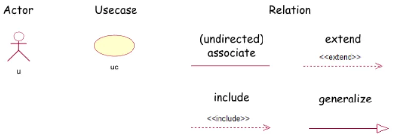
As Figure 5 depicts, usually use case diagram contains three main ele-ments: Actor, Usecase and Relation. An Actor is a person, an organization, or an external system that plays a role in one or more interactions with the system and is drawn as a stick figure. A Usecase describes a sequence of actions that provide something of measurable value to an actor. Use-cases are drawn as horizontal ellipses. Relation shows which Actor carries out which Usecase, or which Usecase includes other Usecase, and use case diagram also includes other Relations between Usecases beyond the simple “include”, such as “extend”, “generalize”. Relation can be directed (signi-fied with an arrow) or undirected, which means the two parts are related with each other. And relation is drawn as solid line (for “associate” and “generalize”) or dashed line (for “include” and “extend”) according to dif-ferent represented meanings.
Actor Usecase
(undirected) associate
include
extend
generalize
u uc
Relation
Figure 5: Elements of use case diagram.
Schema UCD ={
Element PrimitiveString;
ElementEntity{
attributename : String[1];
}
ElementActor extendsEntity {
attributesrc of : Relation[0-*];
attributedest of : Relation[0-*];
}
ElementUsecaseextends Entity{
attributesrc of : Relation[0-*];
attributedest of : Relation[0-*];
}
ElementRelation{
attributename : String[1];
}
ElementUniRelationextends Relation{
attributesrc : Entity[1];
attributedest : Entity[1];
}
ElementBiRelation extendsRelation {
attributesrc : Entity[2];
} }
tiger eating meat
Figure 6: Real case of use case diagram.
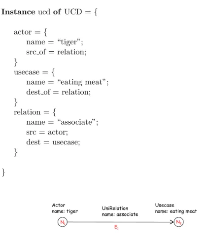
Instance ucdof UCD ={
actor ={
name = “tiger”; src of = relation;
}
usecase ={
name = “eating meat”; dest of = relation;
}
relation ={
name = “associate”; src = actor;
dest = usecase;
}
}
Actor name: tiger
Usecase name: eating meat UniRelation
name: associate
N1 N2
E1
Figure 7: Illustration of InterRep graph of Figure 6.
Figure 7 illustrates the InterRep graph of the given use case diagram. It is composed of two elements shaped as nodes, Actor “tiger” and Usecase “eating meat”, and one element shaped as edge, UniRelation “associate”, from “tiger” to “eating meat”.
The TransAlg part of iGRT will then use the transformation algorithm to transform this normalized graph to UncalRep one. Now let’s see what the UncalRep graph is.
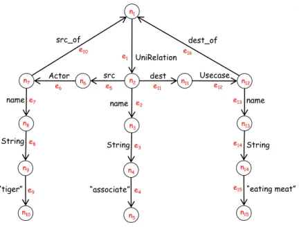
As Figure 8 depicts, the UncalRep graph for the real-world use case
di-agram in Figure 6 is a directed edge-labeled graph (the node’s label “ni”
and edge’s label “ei” are only for explanation, and they are not meaningful
in the real representation). In the UncalRep graph, each element of the InterRep graph is extended to several nodes and edges, with labels to show what the element is, what the element’s attribute’s name is, what the ele-ment’s attribute’s type is and what the eleele-ment’s attribute is. For example,
in Figure 8,{n1, e1, n2} means the element is “UniRelation”, and {e2, n3,
e3, n4, e4, n5} means this attribute has a name attribute “associate”, with
the type “String”. {e5, n6, e6, n7}tells that the “UniRelation” element has
Actor Usecase UniRelation
String
src dest
name
e1
n1
src_of
“associate” e4 String
“tiger”
dest_of
name
String
“eating meat”
n2
name
n3
n4
n5
n6
n7
n8
n9
n10
n11 n12
n13
n14
n15
e2
e3
e5
e6
e7
e8
e9
e10
e11 e12
e13
e14
e15
e16
Figure 8: UncalRep graph of Figure 6.
B. Class Diagram
Class diagram is another useful diagram in the Unified Modeling Lan-guage. It is a type of static structure diagram that describes the structure of a system by showing the system’s classes, their attributes, operations (or methods), and the static relations that exist among the classes.
Figure 9 shows the two main elements of the class diagram: Class and Relation. Class represents both the main objects and interactions in the application and the objects to be programmed. Classes are drawn as boxes which contains three parts: the name of the class, the attributes of the class and the methods or operations the class can take or undertake. Relation depicts the specific types of logical connections found among classes. There are five kinds of relations: associate, aggregate, composite, depend and gen-eralize, each is drawn as a solid/dashed line with different kinds of arrows accordingly.
The schema of class diagram is described as follows. Here the Class’s attributes “attribute” and “operation” themselves are also elements.
Schema CD = {
Element PrimitiveString;
ElementAttribute {
class
(undirected) associate
generalize (undirected)
aggregate
(undirected) composite
depend
Relation
Figure 9: Elements of class diagram.
attributetype : String[1];
}
ElementOperation {
attributename : String[1];
}
ElementClass {
attributename : String[1];
attributeattribute : Attribute[0-*];
attributeoperation : Operation[0-*];
attributesrc of : Relation[0-*];
attributedest of : Relation[0-*];
}
ElementRelation{
attributename : String[1];
}
ElementUniRelationextends Relation{
attributesrc : Class[1];
attributedest : Class[1];
}
ElementBiRelation extendsRelation {
attributesrc : Class[2];
} }
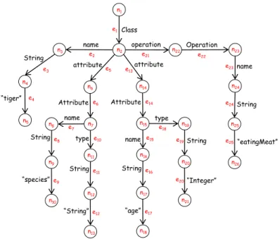
Figure 10 is a simple concrete class diagram in the real world. It only contains one class, with name “tiger”, attributes “species” and “age”, and operation “eatingMeat”. The following is the InterRep graph of the class diagram:
Instance cdof CD = {
attribute1 ={
name = “species”; type = “String”;
}
attribute2 ={
name = “age”; type = “Integer”;
}
operation ={
name = “eatingMeat”;
}
class ={
name = “tiger”; attribute = attribute1; attribute = attribute2; operation = operation;
}
}
Then the UncalRep graph of Figure 10 can be easily given by iGRT as Figure 11 shows.
C. State Diagram
State diagrams are used to give an abstract description of the behavior of a system. This behavior is analyzed and represented in series of events, which could occur in one or more possible states. State diagrams have four main elements which are shown in Figure 12. A state represents a stage in the behavior pattern of an object in the system. An initial state, also called a creation state, is the one that an object is in when it is first created, whereas a final state is one in which no transitions lead out of. A transition is a progression from one state to another and will be triggered by an event that is either internal or external to the object.
The schema of the state diagram is as follows:
attribute Operation Class String operation name e1 n1 e4 String name String “eatingMeat” n2 name n3 n4 n5 n6 n8 n9 n10
n22 n23
n24
n25
n26 e2
e3 e5
e7
e8
e9
e21 e22
e23
e24
e25 “tiger”
n7
Attribute e6
“species” type String n11 n12 n13 e10 e11 e12 “String” name n14 n19 n20 n21 e19 e20
Attribute e14
type String n16 n17 n18 e15 e16 e17 “age” e18 String “Integer” attribute e13 n15
Figure 11: UncalRep graph of Figure 10.
s
InitialState FinalState
State Transition
Figure 12: Elements of state diagram.
Element PrimitiveString;
ElementEntity{
attributename : String[1];
}
ElementInitialState extendsEntity {
attributesrc of : Transition[0-*];
}
ElementFinalState extendsEntity {
attributedest of : Transition[0-*];
}
ElementState extendsEntity{
attributesrc of : Transition[0-*];
attributedest of : Transition[0-*];
}
ElementTransition {
attributename : String[1];
attributedest : Entity[1];
} }
default CAPS_LOCK caps_locked
Figure 13: Real case of state diagram.
Figure 13 is a fragment of a concrete state diagram. It is composed of two states “default” and “caps locked”, and one transition “CAPS LOCK” from the former state to the latter one. This state diagram implies that by doing the “CAPS LOCK” transition, the “default” state can be transformed to the “caps locked” state. Following is the InterRep graph of the state diagram according to the schema:
Instance sdof SD ={
state1 ={
name = “default”; src of = transition;
}
state2 ={
name = “caps locked”; dest of = transition;
}
transition ={
name = “CAPS LOCK”; src = state1;
dest = state2;
}
}
Similarly, the UncalRep graph of the state diagram in Figure 13 can be easily given by iGRT as Figure 14 shows.
State State Transition
String
src dest
name
e1
n1
src_of
“CAPS_LOCK” e4
String
“default”
dest_of
name
String
“caps_locked”
n2
name
n3
n4
n5
n6
n7
n8
n9
n10
n11 n12
n13
n14
n15
e2
e3
e5
e6
e7
e8
e9
e10
e11
e12
e13
e14
e15
e16
Figure 14: UncalRep graph of Figure 13.
graph and UncalRep graph bidirectionally without losing any information.
4
TransAlg in iGRT
In this section, we will explain the mechanism of iGRT’s last part, the TransAlg part. This part targets at doing traceable transformation between InterRep graph and UncalRep graph bidirectionally. We will first introduce the algorithms for general graphs, and then instantiate it by taking a look at how it works on use case diagram.
4.1 General Algorithm
As we have stated before, for real-world graphs, according to the general schema designed, all the properties such as nodes and edges are regarded as elements and their attributes in the InterRep graph. Meanwhile, in the UncalRep graph, all of the elements and attributes are transformed to cor-responding edge-labeled branches.
A. InterRep to UncalRep
For each UncalRep graph, we will scan all the elements one by one, and reconstruct them as two nodes plus one edge. The edge is labeled with the element’s name. For each attribute of the element, if it is primitive type, we will expand it to a new branch with three nodes and three edges. The edges are labeled with the attribute’s name, the attribute’s type and the attribute itself separately. If the attribute’s type is element type, we will first add one edge labeling the attribute’s name, and then check whether the element has been processed yet. For processed element, we will connect the edge to the element’s first node. Else we will process the element using the above procedure and then connect the attribute with it.
In order to keep this transformation traceable, while doing the transfor-mation, we will save the trace information in both parts at the same time. In detail, after transforming the element, we will save the corresponding Un-calRep branch in the element and attribute, and save the element in the first node of the branch. After transforming the element’s attribute, we will save the relevant branch in the element. In this way, all the trace information is kept well.
The pseudo code of the algorithm is as follows:
Algorithm traceable transI2U ( InterRep irg ) {
for each unprocessed element e in irg:
transform(e){
record: e has been processed;
expand it to node1→edge1→node2;
set edge1’s label with e’s name;
save: {node1, edge1, node2}→e;
save: e→node1;
for each attribute a in e: if a’s type is primitive
expand it to edgea→nodea→edgeb→nodeb→edgec→nodec;
set the source of edgea with the e’s node2;
set edgea’s label with a’s name;
set edgeb’s label with a’s type;
set edgec’s label with a’s value;
save: edgea, nodea, edgeb, nodeb, edgec, nodec→a; else if its type is element e*
if e* has been processed
expand it to edgea;
set edgea’s label with a’s name;
set the destination of edgea with e*’s node1;
save: edgea→a;
else
expand it to edgea;
set edgea’s label with a’s name;
set the source of edgea with e’s node2;
transform(e*);
set the destination of edgea with e*’s node1;
save: edgea→a;
}
}
When getting the UncalRep graph by this traceable transformation al-gorithm, we can easily trace back to the InterRep graph again by scanning all the nodes and picking up the InterRep elements saved in them as trace information. Then they all can automatically compose the original InterRep graph. The pseudo code of the trace back algorithm is as follows:
Algorithm back2InterRep ( UncalRep urg ){
create InterRep graph irg;
for each node n in urg:
if find an InterRep element e saved in n add e to irg;
return irg;
}
B. UncalRep to InterRep
The traceable transformation algorithm from UncalRep graph to Inter-Rep graph is quite like a reversion of the previous algorithm. In this algo-rithm, first of all, we will scan all the edges in the UncalRep graph. When
finding one unprocessed edgelwhose label is an element’s name according to
the pre-defined or user-defined graph schema, we will create a corresponding
element e in the InterRep graph. And then we will scan all the branches
below edge l. Here each branch will correspond to one attribute of e as
described in the graph schema. If the type of the attribute is primitive, we
will just compress the branch to an attribute and add it to e. Else if the
not. If so, we will add the processed element as an attribute to element e. Else we will first process the element and then add it as an attribute to e. Trace information is also saved while doing the transformation. When compressing each branch to one element, we will save the element in the branch’s first node, and save the branch in the element at the same time. When compressing the corresponding branch of an attribute, we will save it in the relevant attribute. The pseudo code of the algorithm is as follows:
Algorithm traceable transU2I (UncalRep urg){
for each edge e with unprocessed start node in urg:
transform(e){
record: e’s start node has been processed; if e’s label signifies an element
compress nodea→e→nodeb to element ele;
save: nodea, e, nodeb→ele;
save: ele→nodea;
for each outgoing edge from nodeb oe:
if oe signifies a primitive type attribute pa
compress oe→nodea→edgea→nodeb
→edgeb→nodec to ele’s attribute;
save: oe, nodea, edgea, nodeb, edgeb, nodec→ele; else if oe signifies an element type attribute ea
if ea has been processed
compress ea to ele’s attribute;
save: oe→ele; else
/∗ process oe→nodea→edgea ∗/
transform(edgea)
compress edgea’s corresponding element
to ele’s attribute;
save: oe→ele;
}
}
Similarly, when getting the InterRep graph by this traceable transfor-mation algorithm, we can easily trace back to the UncalRep graph again by scanning the elements and picking up all the UncalRep nodes and edges saved in them as the trace information. Then they all can automatically make up the original UncalRep graph. The pseudo code is as follows:
create UncalRep graph urg;
for each element e in irg:
if find UncalRep nodes n1, n2, ..., ni
and edges e1, e2, ..., ej saved in e
add n1, n2, ..., ni and e1, e2, ..., ej to urg;
return urg;
}
After introducing the general traceable transformation algorithms in TransAlg, let’s see how it can work on the specific graph, use case diagram, in order to have a further understanding.
4.2 An Example
In this part, we again use the use case diagram in Figure 6 as concrete example. As Figure 15 illustrates, when given the InterRep graph in Figure 7 as the input for our TransAlg part, it will start transformation by scanning all the elements. When it meets the element Actor “tiger” (N1), it will
transform it to {n6, e6, n7}, then the “name” attribute is being processed.
Because this attribute’s type is primitive, TransAlg will just expand it to{e7,
n8, e8, n9, e9, n10}. When processing its “src of” attribute, as the type is the
“UniRelation” element and it has not been processed before, TransAlg will
transfer to treat this element (E1). {n1, e1, n2}is first created and then{e2,
n3, e3, n4, e4, n5}is also added corresponding to its “name” attribute. When
processing its “src” attribute, as the attribute’s type is “Actor” element and
it has already been transformed, TransAlg will just add e5 and connect it
to n6. For the “dest” attribute, as its type is “Usecase” element and it has not been processed before, TransAlg will again focus on this element.
Then {n11, e12, n12} and {e13, n13, e14, n14, e15, n15} is added. As the
“dest of” attribute is the processed element “UniRelation”, TransAlg will
just add e16and connect it to n1. After the element Usecase “eating meat” is
processed, TransAlg will add e11and let it point to n11, and now the element
UniRelation “associate” has also been processed. At last, TransAlg will add
e10 and connect it to n11. While doing the transformation, TransAlg will
save the trace information as Figure 15 shows. In the InterRep graph, {n6,
e6, n7, e7, n8, e8, n9, e9, n10, e10} is saved in element N1 and its attributes.
{n1, e1, n2, e2, n3, e3, n4, e4, n5, e5, e11} is saved in element E1 and its
attributes, and {n11, e12, n12, e13, n13, e14, n14, e15, n15, e16} is saved in
element N2 and its attributes. In the other part UncalRep graph, N1 is
saved in n6, N2 is saved in n11 and E1 is saved in n1.
want to trace back to the original InterRep graph, we can just scan all the
nodes in the UncalRep graph and pick up N1, N2 and E1 saved in them.
Then these three elements will make up the InterRep graph.
On the other hand, when given the UncalRep graph in Figure 8 as input, our TransAlg part will start the transformation by scanning all the edges to find one whose label is an element’s name. Here it will first meet e1, then
the element “UniRelation” (E1) is created. By scanning its branch {e2,
n3, e3, n4, e4, n5}, the “name” attribute “associate” is added to E1. When
meeting the branch edge e5, as it represents an unprocessed element “Actor”,
N1 is created, and the “name” attribute “tiger” is added. Again TransAlg
will meet another attribute with element type “UniRelation”, and as it has
already been processed, TransAlg will just add E1 to N1 as the “src of”
attribute. After that, the “Actor” N1 is added as E1’s “src” attribute.
Similarly, TransAlg will regard E1 as N2’s “dest of” attribute and N2 as
E1’s “dest” attribute. The trace information is also saved in both part while doing the transformation.
After getting the InterRep graph, if we want to trace back to the original UncalRep graph, we can just scan all the elements and their attributes in the InterRep graph and find the UncalRep nodes and edges saved in them. Then we can compose the UncalRep graph automatically by using these nodes and edges.
Actor name: tiger
N1——>n6
N2——>n11
E1——>n1
Usecase name: eating meat UniRelation name: associate N1 N2 E1 Actor Usecase UniRelation String src dest name e1 n1 src_of “associate”e4 String “tiger” dest_of name String “eating meat” n2 name n3 n4 n5 n6 n7 n8 n9 n10 n11 n12 n13 n14 n15 e2 e3 e5 e6 e7 e8 e9 e10 e11 e12 e13 e14 e15 e16 Element Actor
n6, e6, n7
Attribute name
e7, n8, e8,
n9, e9, n10
Attribute src_of
e10
Element UniRelation
n1, e1, n2
Attribute name
e2, n3, e3,
n4, e4, n5
Attribute src
e5
Attribute dest
e11
Element Usecase
n11, e12, n12
Attribute name
e13, n13, e14,
n14, e15, n15
Attribute dest_of
e16
tiger eating meat
Figure 15: Transformation between Figure 7 and Figure 8 by TransAlg part.
the ”traceable” attribute and maintain the synchronization of the two kinds of graphs by propagating the graph update between them. In the next section, we will show two useful operations, graph modification propagating and graph query propagating, which help fulfill this synchronization task.
5
Operations for Synchronization
In order to synchronize the real world graph in InterRep and GRoundTram graph in UncalRep, a set of operations need to be provided for this purpose. In this section, we will describe two useful operations based on the trace information saved during the transformation. By these operations, users can keep two graphs being updated at the same time.
5.1 Graph Modification Propagating
In order to make two graphs synchronized, when one kind of the graph is modified, the other kind of the graph should also keep this modification in parallel. In detail, when we modify some elements or attributes in the IntreRep graph, the nodes and edges in the UncalRep graph corresponding to this modified part should also be changed. Meanwhile, changes in the InterRep graph ought to be reflected in the UncalRep graph as well.
This work consists of two main steps, the first step is difference analysis. In this step, we need to compare the original graph and the modified one to extract all the changed part between them. The second step is change impact analysis. After modified part being extracted, we need to recognize the relevant changes in the other kind of the graph by checking the saved trace information.
Here we will explain methodology on propagating two kinds of mod-ification, adding and deleting, from InterRep graph to UncalRep graph. Solutions for propagating modifications of other kinds can easily be worked out by referring to these algorithms.
Suppose we have two graphs, oig and oig+
, being the original InterRep graph and the modified one separately, the modification only includes adding and deleting. By using the traceable transformation algorithm explained before, we have transformed the InterRep graph to UncalRep graph ug, with trace information saved in both parts. Our target is to get the corresponding
modified UncalRep graph ug+
, which exactly matches with oig+
.
ug to get ug+
. For adding operation, we will use the traceable transformation algorithm to transform the modified part to UncalRep graph. When meeting some elements or attributes being treated before, we will just connect the new transformed edge with the existed corresponding part in ug and finally
get ug+
.
For example, Figure 16 shows a graph modification on the use case dia-gram we have mentioned before. Here the relation from “tiger” to “eating meat” is deleted. In order to reflect this modification on the UncalRep graph, first we need to identify all the affected elements and attributes in the InterRep graph related with this change. By checking the graph schema of the use case diagram, we can easily find that there are three places being changed, the UniRelation element “associate”, the “src of” attribute of the Actor element “tiger” and the “dest of” attribute of the Usecase element “eating meat”. They all have been deleted. Then by checking the saved trace information in these three parts, we can easily synchronize the mod-ification to the UncalRep graph by deleting the corresponding nodes and
edges{n1, e1, n2, e2, n3, e3, n4, e4, n5, e5, e10, e11, e16}.
Actor name: tiger
Usecase name: eating meat UniRelation
name: associate
N1 N2
E1 Actor Usecase UniRelation String src dest name e1 n1 src_of
“associate”e4
String “tiger” dest_of name String “eating meat” n2 name n3 n4 n5 n6 n7 n8 n9 n10
n11 n12
n13 n14 n15 e2 e3 e5 e6 e7 e8 e9 e10
e11 e12
e13
e14
e15
e16
Element Actor
n6, e6, n7
Attribute name e7, n8, e8,
n9, e9, n10
Attribute src_of e10
Element UniRelation
n1, e1, n2
Attribute name e2, n3, e3,
n4, e4, n5
Attribute src e5
Attribute dest e11
Element Usecase
n11, e12, n12
Attribute name e13, n13, e14,
n14, e15, n15
Attribute dest_of e16 tiger eating meat
Figure 16: Example of graph modification.
5.2 Graph Query Propagating
As described before, we have presented a bidirectional transformation frame-work between general graphs and the GRoundTram graphs. Here come two problems : one is how to operate on the general graphs; the other one is how to translate the operation on general graphs to the GRoundTram graphs. We solve these two problems by proposing a graph query language iGQL
schema of the specified real world graphs, thenQin iGQL can be
automat-ically translated into queryQ′ in UnQL which queries on the GRoundTram
graph. Since we getQ′, we can use the powerful bidirectional GRoundTram
system to execute the queryQ′.
Figure 17: Overview of Query Translation
Figure 17 gives an overview of the propagating of query Q. The iGRT
framework contains two parts: one is for transforming real world graphs into
GRoundTram graphs; the other is automatically transformation of queryQ
intoQ′.
Here let us take a look at a simple example for the use case diagrams illustrated in Figure 6. If we want to select the actor whose name is “tiger”
in the use case diagrams as in Figure 7, we can write a queryQ like this:
Q = select {$a }
where{Actor : $a} in $db
$a.name = “tiger”
Query Q is written based on the schema UCD of the usecase graph.
From the schema, we can see that Actor is the name of an element. The
Actor has anameattribute, asrc of attribute and adest ofattribute. The
query is aiming at choosing actors whose name is “tiger”.
In order to get the answer of Q by iGRT, we need to translate query
Q into query Q′ which is viewed as the input query of the GRoundTram
system. Figure 8 illustrates the representation of ausecasegraph in Figure
7 in GRoundTram system. The queryQ′ is expressed as follows:
Q′ =select{ $a}
where{ ∗.Actor : $a} in $db
So in fact we execute queryQ′ on the GRoundTram system and then get
the result through the bidirectional iGRT framework. When comparing Q′
with Q, the main difference is that query Q does not give the information
of types of each attribute, while in Q′ the type of attribute also considered
in the Query. This is because the graph data model of GRoundTram is for semi-structured data. So the type of attributes has been added as an edge label of the graph. This is just a simple case, the graph structure may also changed in complex situations.
6
Implementation
So far we have introduced all the concepts and methodologies used in iGRT. In this section, we will explain the technical details of iGRT.
We have implemented iGRT based on the eclipse platform. Figure 18 is the package explorer of iGRT. From the picture, we can see that it is composed of three modules, interRep, transAlg and uncalRep, responsible for graph representations and transformation algorithms.
Figure 18: Package explorer of iGRT.
6.1 InterRep
several attributes, represented by class “Attribute”, and “Attribute” has name, type and number.
Figure 19: Code fragment of class ”Schema”.
As described in Figure 20, class “Instance” signifies the instance of the schema. It still has some elements, and each element has some attributes. Here the element and attribute are also represented by class “Element” and “Attribute”. This is the reason why they are in the “common” package. In order to separate them from being used in schema or in instance, they have one attribute called “role” to indicate their position.
Figure 20: Code fragment of class ”Instance”.
Figure 21: Code fragment of class ”EmbeddedScheInst”.
6.2 UncalRep
This module is responsible for representing the graphs in GRoundTram. Figure 22 is a code fragment of class “UncalRep”. It is very much simi-lar to graph representation. There are several nodes and edges inside it, represented by class “UncalNode” and “UncalEdge”. And it has attribute “schema” to point out with which kind of graph schema it relates. As un-calRep graph is directed graph with edge labeled, “UncalNode” only has attribute “id” to identify different nodes, and “UncalEdge” has attribute “id” and “label”, representing the label of the edge. One additional thing to mention in class “UncalRep” is that by calling the method “toDot”, we can transform the UncalRep graph to graph in GRoundTram with its internal representation.
6.3 TransAlg
This module serves as the transformation algorithm part of iGRT. It is com-posed of two classes, “TraceableI2U” and “TraceableU2I”, corresponding to the transformation from InterRep graph to UncalRep graph and the reversed one.
Figure 22: Code fragment of class ”UncalRep”.
used in “traceableI2U”. The “TraceableU2I” is quite the similar, so we will not explain it here.
Figure 23: Code fragment of class ”TraceableI2U”.
7
Conclusion
References
[1] Atlas group, km3: Kernel metametamodel manual,
http://www.eclipse.org/gmt/atl/doc.
[2] C. Brabrand, A. Møller, and M. Schwartzbach. Dual syntax for xml
languages. Information Systems, 33(4):385–406, 2008.
[3] P. Buneman, M. Fernandez, and D. Suciu. Unql: a query language
and algebra for semistructured data based on structural recursion. The
VLDB JournalThe International Journal on Very Large Data Bases,
9(1):76–110, 2000.
[4] Y. Chen and Z. Hu. Ao software behavior model evolution and syn-chronization: A bidirectional graph transformation approach. Technical report.
[5] K. Czarnecki, J. Foster, Z. Hu, R. L¨ammel, A. Sch¨urr, and J.
Ter-williger. Bidirectional transformations: A cross-discipline perspective.
Theory and Practice of Model Transformations, pages 260–283, 2009.
[6] S. Hidaka, Z. Hu, K. Inaba, H. Kato, K. Matsuda, and K. Nakano. Bidi-rectionalizing structural recursion on graphs. Technical report, Tech-nical Report GRACE-TR09-03, GRACE Center, National Institute of Informatics, 2009.
[7] S. Hidaka, Z. Hu, K. Inaba, H. Kato, K. Matsuda, and K. Nakano.
Bidirectionalizing graph transformations. InACM Sigplan Notices,
vol-ume 45, pages 205–216. ACM, 2010.
[8] S. Hidaka, Z. Hu, K. Inaba, H. Kato, and K. Nakano. Groundtram version 0.9.2 user manual.
[9] S. Hidaka, Z. Hu, K. Inaba, H. Kato, and K. Nakano. Groundtram: An integrated framework for developing well-bahaved bidirectional model transformations. August 2011.
[10] S. Kato and K. Hu. Towards bidirectional transformations on ordered graphs.
[11] I. Sasano, Z. Hu, S. Hidaka, K. Inaba, H. Kato, and K. Nakano. Toward
bidirectionalization of atl with groundtram. Theory and Practice of
Model Transformations, pages 138–151, 2011.
[13] Y. Yu, Y. Lin, Z. Hu, S. Hidaka, H. Kato, and L. Montrieux.
blinkit: Maintaining invariant traceability through bidirectional
transformations–a technical report. The Open University, Tech. Rep.

![Figure 9: Elements of class diagram. attribute type : String[1];](https://thumb-ap.123doks.com/thumbv2/123deta/8631254.449567/15.892.203.639.106.1098/figure-elements-class-diagram-attribute-type-string.webp)